SQL-Engineering-Handbook
01 · Advanced GROUP BY
🏠 Module Home · 🗂️ Handbook Home · Next → 02 Multiple Aggregations
Module: 02 — Advanced Aggregations Domain used in this file: Human Resources (
employees,departments,locations) Companion file:01_ADVANCED_GROUP_BY.sql
Introduction
A single-column GROUP BY answers one question: “what’s the total per category?” The moment a stakeholder asks for a total per category, broken down by a second category, you need multi-column and nested grouping — the subject of this file.
This is the single most common upgrade a beginner analyst has to make: moving from “total sales per region” to “total sales per region, per month, per product category.” The SQL mechanism barely changes. What changes is your responsibility to reason correctly about grain — exactly what one output row represents.
Concept Overview
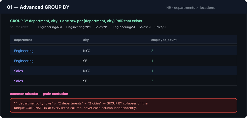
GROUP BY col1, col2, ... collapses rows into groups defined by the unique combination of every listed column — not each column independently. GROUP BY department, city does not produce “one group per department plus one group per city.” It produces one group per (department, city) pair that actually exists in the data.
This combination is called the grain of the result set. Every aggregate function in the SELECT list (COUNT, SUM, AVG, etc.) is computed within that grain, one value per group.
Business Motivation
An HR analytics team is asked: “Give me headcount by department, and also tell me how that breaks down by office location.” A single-column GROUP BY department cannot answer the location part. A single-column GROUP BY location cannot answer the department part. Only grouping by both columns together produces a table where each row is a legitimate, addressable business unit: “8 people in Engineering, in the Nagpur office.”
This is the pattern behind virtually every cross-tabulated business report: revenue by region and quarter, tickets by severity and team, orders by channel and payment method.
Why This Feature Exists
Relational databases store data in its most granular, transactional form — one row per employee, one row per order line. Businesses almost never think at that grain; they think in aggregates, at whatever combination of dimensions matters for the decision being made. GROUP BY with multiple columns is the mechanism that lets the same underlying table answer questions at many different levels of granularity, without needing a separate pre-built table for every possible breakdown.
Real Company Examples
- Workday / BambooHR-style HRIS reporting — headcount dashboards broken down by department, location, and employment type simultaneously.
- Retail chains — same-store sales reported by region and by week, in one management report.
- Telecom operators — customer churn reported by plan tier and by acquisition channel together, to isolate which combination is actually driving losses.
Business Problems Solved
- Headcount and organizational reporting across more than one dimension at once
- Identifying which combination of factors (not just one factor alone) drives a metric
- Producing cross-tabulated, matrix-style reports without a spreadsheet pivot table
- Feeding BI tools a pre-aggregated table at the exact grain a dashboard filter needs
Visual Explanation
Grouping by a single column collapses rows into one bucket per value:
GROUP BY department
┌─────────────┐        ┌───────────────────────┐
│ Engineering │──┐     │ Engineering  →  8 rows │
│ Engineering │──┼──▶  └───────────────────────┘
│ Engineering │──┘     ┌───────────────────────┐
│ Sales       │──┐     │ Sales        →  5 rows │
│ Sales       │──┘     └───────────────────────┘
Grouping by two columns collapses rows into one bucket per combination:
GROUP BY department, city
┌─────────────────────────┐    ┌─────────────────────────────────┐
│ Engineering | Nagpur     │──┐ │ Engineering, Nagpur   →  5 rows │
│ Engineering | Nagpur     │──┘ └─────────────────────────────────┘
│ Engineering | Pune       │──┐ │ Engineering, Pune     →  3 rows │
│ Engineering | Pune       │──┘ └─────────────────────────────────┘
│ Sales       | Nagpur     │──┐ │ Sales, Nagpur         →  5 rows │
│ Sales       | Nagpur     │──┘ └─────────────────────────────────┘
Notice the grain got finer — more, smaller groups — the moment a second column was added.
Syntax
SELECT
    col1,
    col2,
    AGG_FUNCTION(col3) AS metric_alias
FROM table_name
GROUP BY col1, col2
[HAVING aggregate_condition]
[ORDER BY col1, col2];
Rule: every column in SELECT that is not wrapped in an aggregate function must appear in GROUP BY. This applies in strict SQL modes (PostgreSQL always; MySQL under ONLY_FULL_GROUP_BY, which is the default since MySQL 5.7).
Detailed Walkthrough
SELECT
    d.dept_name,
    l.city,
    COUNT(DISTINCT e.emp_id) AS total_employees
FROM employees AS e
JOIN departments AS d ON e.dept_id = d.dept_id
JOIN locations  AS l ON d.location_id = l.location_id
GROUP BY d.dept_name, l.city
ORDER BY d.dept_name, l.city;
- The
FROM/JOINclauses build the full detail row set — one row per employee, carrying their department and city. GROUP BY d.dept_name, l.citycollapses that detail set into one row per (department, city) combination actually present in the data.COUNT(DISTINCT e.emp_id)computes the metric within each group.ORDER BYis applied last, after aggregation, to sort the final report — not the raw rows.
Production Workflow
Multi-column GROUP BY queries typically sit in a scheduled reporting job or a dbt model: raw HR/transactional tables are joined and grouped at a fixed grain, the result is materialized into a summary table, and the BI layer queries that summary table instead of re-aggregating the full history on every dashboard load.
Analytics Engineering Perspective
- Decide the grain before writing the query, and write it as a comment (
-- grain: one row per department, city). This is the single habit that prevents most multi-columnGROUP BYbugs. - Joins before grouping can silently change your grain. A one-to-many join (e.g., employees to a
certificationstable where an employee can have several rows) will inflate counts unless you aggregate withCOUNT(DISTINCT ...)or pre-aggregate the many side first. - Every additional
GROUP BYcolumn is a promise to consumers of the report that this breakdown is meaningful and stable — don’t add dimensions “just in case,” since it changes the grain contract of the output.
Performance Considerations
- A composite index on the
GROUP BYcolumns (e.g.,(dept_id, location_id)) lets the engine use an index-based grouping strategy instead of a full sort/hash of the entire joined result. - Grouping by high-cardinality combinations (e.g.,
emp_id, hire_date) can produce a result set nearly as large as the source data — confirm the expected number of groups before running against a large table. - Filter with
WHEREbefore theJOIN/GROUP BYwherever possible; reducing the row count before aggregation is always cheaper than aggregating everything and filtering withHAVINGafterward.
Edge Cases
- NULL grouping keys. A
NULLin aGROUP BYcolumn forms its own group (e.g., employees with nomanager_idgroup together underNULL, not one row per person). - Join fan-out. If
departmentswere joined to a hypothetical multi-rowdept_budget_linestable before grouping,COUNT(e.emp_id)(withoutDISTINCT) would over-count employees. Always sanity-check counts after adding a new join. - Empty groups don’t appear.
GROUP BYonly returns combinations that exist in the joined data — a department with zero employees in a given city will not appear as a zero row; it simply won’t appear at all. If you need explicit zeros, you need an outer join against a dimension table listing all valid combinations.
Common Mistakes
- Adding a column to
SELECTand forgetting to add it toGROUP BY(or vice versa). - Using
COUNT(col)instead ofCOUNT(DISTINCT col)after a join that can produce duplicate rows per entity. - Assuming
GROUP BYpreserves the input row order — it does not; always add an explicitORDER BYfor a stable, presentable report. - Filtering the aggregated metric with
WHEREinstead ofHAVING(covered in depth in later topics of this module).
Best Practices
- State the intended grain in a comment above every non-trivial
GROUP BYquery. - Alias every grouped and aggregated column with a clear business name.
- Use
COUNT(DISTINCT primary_key)by default whenever a join is present in the query, unless you have specifically verified the join is one-to-one. - Keep
GROUP BYcolumn order consistent withSELECTandORDER BYfor readability, even though SQL does not require it.
Interview Questions
- What determines a “group” when
GROUP BYlists more than one column? The unique combination of values across all listed columns — not each column independently. - Why might
COUNT(emp_id)return a higher number than the actual headcount after a join? A one-to-many join (e.g., to a table with multiple rows per employee) duplicates employee rows before aggregation;COUNT(DISTINCT emp_id)corrects this. - What happens to rows with a
NULLvalue in aGROUP BYcolumn? They form their own group underNULL, rather than being excluded or erroring. - Why does adding a second
GROUP BYcolumn typically increase the number of output rows? It makes the grain finer — you’re now grouping by combinations rather than single values, which almost always produces more, smaller groups. - How would you get a department to appear with zero headcount in a given city, if no employees currently match?
GROUP BYalone won’t show it; you need an outer join against a complete dimension table of valid department/city combinations, withCOALESCE(COUNT(...), 0).
Summary
Multi-column GROUP BY is single-column GROUP BY applied to a combination of dimensions instead of one. The mechanism is identical; the responsibility that grows is reasoning correctly about grain — what one row of your output actually represents — especially once joins are involved and row counts can silently inflate before aggregation ever runs.
Practice Challenges
- Write a query returning employee count per department and per manager, in one result set.
- Extend the department/city report in this file to also show the earliest hire date per (department, city) combination.
- Find every (department, city) combination with zero employees, using an outer join against a full list of valid combinations.
- Rewrite the “highest headcount department” scenario in the companion SQL file without a subquery, using only
ORDER BYandLIMIT, and explain the tradeoff versus the subquery version. - Produce a report of employee count by department, city, and whether the employee has a manager — three grouping dimensions in one query.
Further Reading
- PostgreSQL Documentation — GROUP BY and HAVING
- MySQL 8.0 Reference Manual — GROUP BY Handling
- Microsoft Learn — Aggregate Functions (Transact-SQL)
◀ Previous: Module README · Next ▶ 02_MULTIPLE_AGGREGATIONS.md