SQL-Engineering-Handbook

04 — CTEs With Aggregations

Aggregation pipeline: WHERE vs HAVING

In this file: applying COUNT, GROUP BY, and HAVING on top of a CTE join chain to answer workforce-concentration questions, and the precise difference between filtering rows and filtering groups.

Business Question

Which departments and cities have the highest workforce concentration?

Why This Matters

Joining tables together (File 03) gets you a wide, row-level report. But most business questions aren’t about individual rows — they’re about counts, totals, and thresholds across groups: “which departments have more than one employee,” “how many people work in each city.” This file layers GROUP BY aggregation on top of the exact same CTE join chain from File 03, which is the normal shape of an analytical query: prepare → join → aggregate.

SQL Solution

See 04_CTE_Aggregation.sql for all five queries.

WITH emp_cte AS (
    SELECT emp_id, emp_name, dept_id
    FROM employes
),
dept_cte AS (
    SELECT dept_id, dept_name
    FROM departments
)
SELECT
    d.dept_id,
    d.dept_name,
    COUNT(e.emp_id) AS num_of_emp
FROM emp_cte e
JOIN dept_cte d ON e.dept_id = d.dept_id
GROUP BY d.dept_name, d.dept_id
HAVING COUNT(e.emp_id) > 1;

Explanation

CTEs prepare the employee, department, and location data exactly as in File 03. Aggregation is then applied in the outer query using COUNT and GROUP BY — the CTEs themselves stay simple, row-level building blocks; all the aggregation logic lives in one place, the final SELECT.

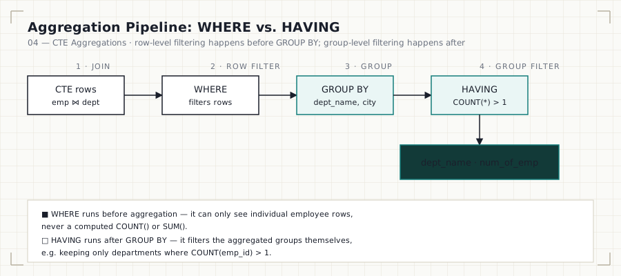
The critical distinction this file tests is when each filter runs:

Clause	Filters	Runs	Can reference `COUNT()`?
`WHERE`	Individual rows	Before `GROUP BY`	No
`HAVING`	Aggregated groups	After `GROUP BY`	Yes

WHERE never sees an aggregate — by the time WHERE runs, no grouping has happened yet. HAVING exists specifically because SQL needs a way to filter on values (like COUNT(emp_id) > 1) that only exist after aggregation.

Finding

The analysis identified employee counts per department and per city, surfacing exactly which departments and cities carry the most headcount. Filtering with HAVING count(e.emp_id) > 1 isolated departments with more than one employee — a filter that would be impossible to express in a WHERE clause, since WHERE cannot see the result of COUNT().

Common Mistakes

Missing a column in GROUP BY — every non-aggregated column in the SELECT list must also appear in GROUP BY (d.dept_name, d.dept_id here, not just one of the two).
Using COUNT(*) when COUNT(e.emp_id) is intended — after a LEFT JOIN (see File 05), COUNT(*) counts the joined row even when e.emp_id is NULL, silently inflating the result.
Filtering aggregates with WHERE instead of HAVING — this simply won’t parse, since WHERE COUNT(e.emp_id) > 1 references an aggregate before one exists.
Forgetting that HAVING can filter on an aggregate expression that isn’t even in the SELECT list — the two don’t have to match.

Interview Tips

“What’s the difference between WHERE and HAVING?” is one of the most asked SQL interview questions, and the correct answer is about execution order, not just syntax position: HAVING is evaluated after aggregation, WHERE is evaluated before it. A strong answer states this explicitly rather than just saying “HAVING is for groups.”

Practice Questions

Find departments with more than 2 employees.
Find the city with the lowest employee count.
Combine both: find cities with more than one department and more than one employee — requires two conditions in the same HAVING clause.

Previous: 03_CTE_Joins.md · Next: 05_Buisness_CTEs.md — turning these aggregates into classified, decision-ready business insights.

This site is open source. Improve this page.