SQL-Engineering-Handbook

03 · City Analysis

Difficulty: Intermediate · Estimated time: 15 min Schema: 00_Sample_Schema.sql

Introduction

Same shape as Lesson 02 (CASE over an aggregate), applied to a multi-table join across locations → departments. This lesson focuses on what happens to CASE classification when the underlying join can fan out or drop rows.

Learning Objectives

• Apply CASE after a GROUP BY that spans two joined tables
• Recognize when JOIN choice (INNER vs LEFT) silently changes classification results
• Use CASE output to drive business decisions (expansion planning)

Business Context

Expansion and resource-allocation decisions (“should we open a second office in this city?”) are often driven by exactly this kind of department-concentration metric.

SQL

See 03_City_Analysis.sql.

Engineering Notes

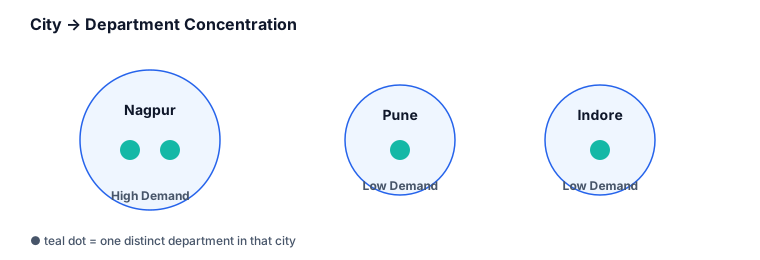
• COUNT(DISTINCT d.dept_id) > 1 is a binary classifier (High/Low Demand) — a good reminder that CASE doesn’t need 3+ branches to be useful; sometimes a clean boolean label is exactly what’s needed instead of a raw count.
• Because this is an INNER JOIN, a city with zero departments (e.g. a new office location added to locations before any department is assigned) won’t appear in the result at all — not even as “Low Demand.” This is the same trap as Lesson 02, worth internalizing because it recurs constantly in real reporting.

Best Practices

• When a CASE threshold is a single cutoff (High vs Low), consider naming the cutoff as a well-known business term in the alias (city_status) and documenting the exact number (> 1) in a comment — thresholds drift, and future maintainers need to know why 1 was chosen, not just that it was.

Common Mistakes

• Assuming “Low Demand” means “we checked and it’s low” — with an INNER JOIN, cities that never got any department at all are invisible, which is a different (and often more urgent) business situation than “low but present.”

Interview Questions

1. Why might a city with genuinely zero departments not appear in this report at all?
2. How would you rewrite the query so every city always appears, even with zero departments?

Answers

1. The `INNER JOIN` between `locations` and `departments` requires a match; a city with no departments produces no joined rows and is dropped before `GROUP BY` even runs. 2. Switch to `LEFT JOIN locations l ... departments d ON l.location_id = d.location_id`, and wrap the count with `COALESCE(COUNT(d.dept_id), 0)` so it doesn't null out.

Cross References

• Previous: 02_Department_Categorization.md
• Next: 04_Employee_Labelling.md

This site is open source. Improve this page.